Predict Uncertainty with Monte Carlo Simulations

Motivation & Goals

In this article we’ll look at how we can use the Monte Carlo method to simulate processes that contain a flow of probabilities. If the process is simple we may be able to calculate the probability of some event deterministically. But what if a decision you might take in one month depends on a combination of a few uncertain events. Your decision then in turn triggers uncertain events and so on until you arrive at a point in time where the sequence of events and decisions have led to a profit - or a loss. To calculate the probability of making a profit in this example we need a new set of tools.

In a moment we’ll run two Monte Carlo analyses using NumPy. First to simulate a robot that doesn’t know exactly how far it travels in which direction. And then to predict a company’s cash-flow. Once we’ve finished the simulations we’ll look at ways to interpret and visualize the results.

Robotic Car ebook

Our step-by-step guide to building a self-driving model car that can navigate your home. Learn all the algorithms and build a real robotic car using a Raspberry Pi.

Sign up now to get exclusive early access and a 50% discount.

We don't spam and you can unsubscribe anytime. Learn more about how we handle your data.

What is Monte Carlo?

Processes involving events that occur with certain probabilities can become so complex that they become impractical or even impossible to solve analytically. Monte Carlo methods get rid of this analytical complexity by simulating single experiments with randomness over and over and over again. In the end you get the results from tens or hundreds of thousands of distinct experiments. These concrete results can easily be turned into interpretable statistics.

Monte Carlo methods were thought up in the Manhattan project partly inspired by the new computational powers that were available back then. For the first time in history it was possible to run a huge amount of calculations in a short time. This made Monte Carlo feasible in the first place. Now it’s often used in physics, mathematics and computer science problems - which is another way of saying it’s used everywhere. As David Silver once said in one of his lectures, "I only get this one stream of data that we call life." - A Monte Carlo simulation gets thousands of possible streams of data. Much like in one of the Black Mirror episodes from season 4. (Don’t want to spoiler you - so no more details)

Using NumPy for Monte Carlo

Before diving into real simulations let’s try out ways to speed up our code so our simulations run fast. This will allow you to iterate quickly on your models. In the first code snippet we calculate the mean of 10 million random numbers.

sum_x = 0
for i in range(int(1e7)):
    x = np.random.rand()
    sum_x += x
print(sum_x / 1e7)  # ~0.5

This code uses a loop that runs 10 million times. Inside the loop it generates a random number using NumPy. It then uses Python code to sum them up and to divide the sum by 10 million to get the expected mean of 0.5. Running this code takes about 6 to 7 seconds on my laptop. Given the simplicity of these calculations that’s quite a lot.

Fortunately there is a quicker and more elegant way: Using NumPy arrays.

x = np.random.rand(int(1e7))  # x is an array containing 10 million random numbers
print(np.mean(x))  # ~0.5

We can tell np.random.rand() that instead of generating a single number it should populate a 10-million-element array with random numbers. This NumPy array has a method to calculate the mean. The above code takes about 0.16 seconds and only has 2 lines of code.

NumPy achieves this speedup by using the efficient data structure ndarray which only holds elements of a single type and is written in C. Take a look at the NumPy docs to see all methods of ndarray.

Another important method for vectorized implementations is np.where(). This replaces if-clauses inside a loop.

Turning this running 6 seconds:

sum_x = 0
for i in range(int(1e7)):
    if np.random.rand() > 0.9:
        sum_x += 1
print(sum_x / 1e7)  # ~0.1

Into this running 0.25 seconds:

x = np.random.rand(int(1e7))
condition = x > 0.9  # boolean ndarray containing 10 million entries
results = np.where(condition, 1, 0)
print(np.mean(results))  # ~0.1

With these two code snippets you know the basics of vectorized implementations and are ready for some real simulations.

Two Examples

We’ll look at two examples. One is taken from robotics and is visually quite intuitive: We want to estimate the uncertainty of a robot’s position after it moves across a room.

In the second example we’ll try to predict whether a company will run out of money over the next ten years.

Feel free to follow one or both examples.

Uncertain Locations of a Robot

You can find the complete code of this example at https://github.com/databriefing/article-notebooks/blob/master/monte-carlo-simulations/robot.ipynb

The premise of this example is that a robot drives around in a room. We can tell it to move a certain distance and to steer in a certain direction. When we tell it to go 10 units the real distance and direction travelled will deviate. So for each simulated step we draw the real distance and real angle from a normal distribution. We use a vectorized implementation:

def go_step(distance_mean, distance_std, angle_mean, angle_std):
    """Calculates deltas in the x and y direction."""
    distances = np.random.normal(distance_mean, distance_std, size=(N_SIMULATIONS))
    angles = np.random.normal(angle_mean, angle_std, size=(N_SIMULATIONS))
    dx = distances * np.cos(np.deg2rad(angles))
    dy = distances * np.sin(np.deg2rad(angles))
    return dx, dy

It’s a good idea to put the real sampling operations in a method that we can call repeatedly. Then we only have to define the starting positions in x and y which itself has a small uncertainty and a matrix to store all positions of all robot simulations of all steps.

x = np.random.normal(60, .3, size=(N_SIMULATIONS))
y = np.random.normal(0, .3, size=(N_SIMULATIONS))
N_STEPS = 19
points = np.zeros((N_STEPS, N_SIMULATIONS, 2))
# Define coordinates at step 0
points[0,:,0] = x
points[0,:,1] = y

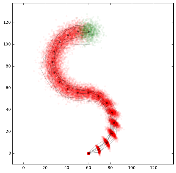
Now we run the simulation for 19 steps. The most complicated part of this is that we first want the robot to turn left and then to turn right. Finally we use a helper function to plot all points.

for i in range(1, N_STEPS):
    # Calculate absolute heading of current step
    heading = 20 * i
    # Turn right after step 9
    if i > 9:
        heading = 360-heading
    # Go one step of distance 10 in the caculated direction.
    dx, dy = go_step(10, 0.1, heading, 10)
    x, y = x+dx, y+dy
    points[i,:,0] = x
    points[i,:,1] = y

plot_points(points)

We also pick 10 different simulation runs and plot their complete paths. This is to visualize the different paths a single robot could take. We have really simulated paths on the level of single robots. The longer the robots travel the more their paths diverge from each other which is exactly what we’ve expected.

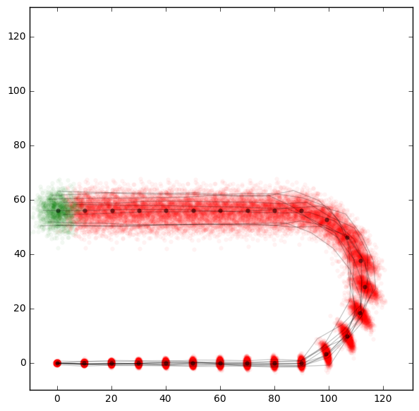
In the example you can also find code for a more complicated robot model. As long as it goes straight it can measure the distance and angle travelled quite accurately. But in a curve the heading measurement will get more error-prone due to random drift on unknown ground. We can see this nicely in the following plot.

Predicting Cash Flow

You can find the complete code of this example at https://github.com/databriefing/article-notebooks/blob/master/monte-carlo-simulations/company_cashflow.ipynb

In this example we want to calculate the risk for a company to run out of cash. First we make a few assumptions to build a simple model of a company.

• Revenue growth year on year is 5% with a standard deviation of 5%-points
• We have an internal profit margin target of 7%
• If we miss this target we reduce the expenses accordingly
  • We might not be able to reduce fixed expenses immediately so with 25% probability expenses remain unchanged
• If we exceed the targeted profit margin we increase expenses
  • Same here. Don’t change with a probability of 25% because we might not be able to e.g. hire more people immediately
• Our single biggest customer generates between 15 and 30% of revenue
• Yearly chance of losing the biggest customer is 10%

Now let’s put all these assumptions into code. Notice how easy it is to sample huge amounts of data points from these distributions with NumPy.

revenue_growth = np.random.normal(1.05, 0.05, size=(N_YEARS, N_SIMULATIONS))
can_change_expenses = np.random.rand(N_YEARS, N_SIMULATIONS) < 0.75  # boolean
biggest_customer_share = np.random.uniform(0.15, 0.4, size=(N_YEARS, N_SIMULATIONS))
biggest_customer_leaves = np.random.rand(N_YEARS, N_SIMULATIONS) < 0.1  # boolean

np.random.rand(N_YEARS, N_SIMULATIONS) < 0.75 is a quick way of getting a boolean array where 75% of the elements are true.

We initialize container matrices to store all our calculated values.

revenues = np.zeros((N_YEARS, N_SIMULATIONS))
profits = np.zeros((N_YEARS, N_SIMULATIONS))
expenses = np.zeros((N_YEARS, N_SIMULATIONS))
cash = np.zeros((N_YEARS, N_SIMULATIONS))

And finally we loop through the years. This is very fast as we’ve vectorized the calculations across the simulations and only loop through 10 years. The other way round would be much slower.

for i in range(N_YEARS):
    if i == 0:
        # first year
        prev_revenue = REVENUE_START * np.ones(N_SIMULATIONS)
        prev_expenses = EXPENSES_START * np.ones(N_SIMULATIONS)
        prev_cash = CASH_START * np.ones(N_SIMULATIONS)
    else:
        prev_revenue = revenues[i-1,:]
        prev_expenses = expenses[i-1,:]
        prev_cash = cash[i-1,:]
    prev_expenses_target = prev_revenue * (1 - PROFITMARGIN_TARGET)
    revenues[i,:] = prev_revenue * revenue_growth[i,:]
    expenses[i,:] = np.where(can_change_expenses[i,:], prev_expenses_target, prev_expenses)
    revenue_from_biggest_customer = biggest_customer_share[i,:] * revenues[i,:]
    revenues[i,:] = np.where(
        biggest_customer_leaves[i,:],
        revenues[i,:] - revenue_from_biggest_customer,
        revenues[i,:]
    )
    profits[i,:] = revenues[i,:] - expenses[i,:]
    cash[i,:] = prev_cash + profits[i,:]

One way to visualize the results is through a plot of each year’s confidence intervals. The function np.percentile comes in quite handy for this.

plt.figure(figsize=(10, 7))
plt.fill_between(np.arange(N_YEARS), *np.percentile(cash, [2.5, 97.5], axis=1), facecolor='b', alpha=0.1, label='95%');
plt.fill_between(np.arange(N_YEARS), *np.percentile(cash, [15, 85], axis=1), facecolor='r', alpha=0.1, label='70%');
plt.plot(np.percentile(cash, 50, axis=1), c='k');
plt.legend()
plt.title('Confidence Intervals of cash amount')
plt.xlabel('Year')
plt.ylabel('Cash');

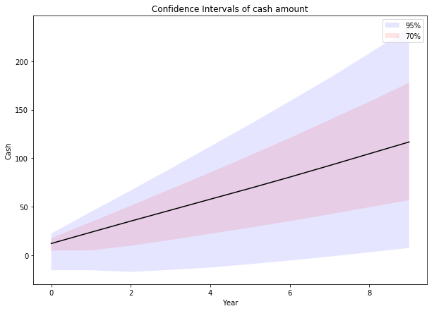
As you can already see with 70% probability we barely make it and with 95% probability we may have negative cash for a long time. Let’s get some numbers for this. I like to think about three probabilities: 51, 95 and 99%. The question we’re asking is, “What amount of money will we have at least with a probability of X%?”

for i in [51, 95, 99]:
    print('With {}% probability cash is always more than: {: 3.2f}'.format(
            i, np.percentile(cash, 100-i, axis=1).min()))

Giving us:

• With 51% probability cash is always more than: 12.15
• With 95% probability cash is always more than: -11.00
• With 99% probability cash is always more than: -28.04

The beauty of this approach is it doesn’t tell you what to do. I like to expect the 51% or 60% value, to prepare for the 95% value and to at least think about the 99% probable outcome. Other people may be more risk-averse or risk-affine and might look for other probabilities.

In this case and for me it would mean to talk to several banks about an overdraft facility early on.

Where to go from here

Optimize input values

What if you have constraints? For example if your cash can never ever fall below a certain amount you might have to tweak input values.

Sensitivity Analysis

The other question is which of your parameters change the end result most directly. You can conduct an automatic sensitivity analysis or systematically try out different input parameters. In the cash-flow example this seems to be the size of the biggest customer and the likelihood of them leaving. So these two aspects might be effective areas to focus resources on.

In the robot example the question would be whether you should focus on making the angle-measurements more accurate by adding more sensors and how this would affect the certainty of the robot’s position after driving around for a while.

Monte Carlo analysis is only ever as good as the models it’s based on but it can help you make uncertainty quantifiable.